
Linkedin Instagram Facebook X-twitter Case Study Automating the generation of javascript expressions with Pre-Trained AI Models Challenge Developing a user-friendly…
Bayesian Machine Learning is a powerful and flexible approach that uses probability theory to model uncertainty in machine learning. Unlike frequentist methods that provide point estimates for parameters, Bayesian methods treat parameters as random variables with their own distributions. This allows us to incorporate prior knowledge and update our beliefs as new data becomes available.
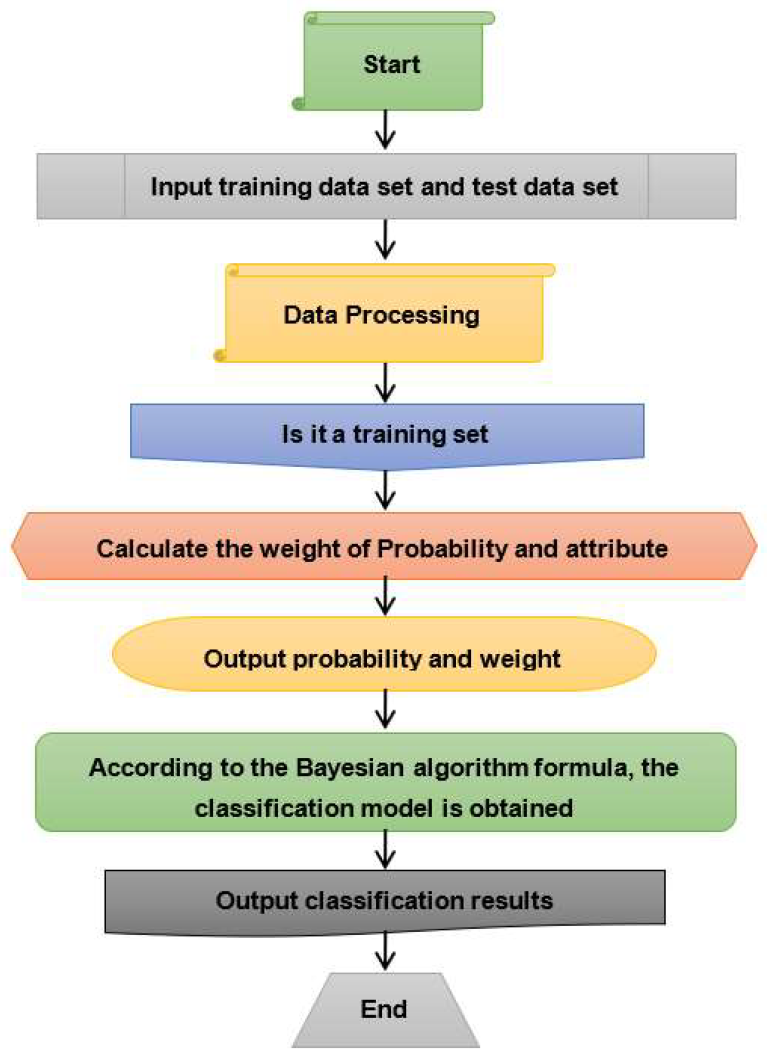
Bayes’ Theorem is the cornerstone of Bayesian inference. It relates the conditional and marginal probabilities of random events. Mathematically, it is expressed as:
\[P(\theta \mid D) = \frac{P(D \mid \theta) \cdot P(\theta)}{P(D)}\]
where:
• \(\theta\) represents the model parameters.
• \(D\) represents the observed data.
• \(P(\theta \mid D)\) is the posterior probability, the probability of the parameters given the data.
• \(P(D \mid \theta)\) is the likelihood, the probability of the data given the parameters.
• \(P(\theta)\) is the prior probability, the initial belief about the parameters.
• \(P(D)\) is the marginal likelihood or evidence, the total probability of the data.
The prior \(\theta \) represents our initial belief about the parameters before observing any data. Priors can be informative or non-informative:
• Informative Priors: Incorporate existing knowledge about the parameter.
• Non-informative Priors: Used when there is no prior knowledge, typically uniform distributions.
For example, if we have prior knowledge that a parameter \(\theta \) follows a normal distribution,
we can use:
\[ \theta \sim \mathcal{N}(\mu_0, \sigma_0^2) \]
where \(\mu_0\) and \(\sigma_0^2\) are the mean and variance of the prior distribution.
The likelihood function \(P(D | \theta)\) represents the probability of observing the data given the parameters. For instance, if our data follows a normal distribution:
\[ D_i \sim \mathcal{N}(\theta, \sigma^2) \]
the likelihood for a dataset
\[ P(D | \theta) = \prod_{i=1}^n \mathcal{N}(D_i | \theta, \sigma^2) \]
The posterior distribution \(P(\theta \mid D)\) combines the prior and the likelihood to update our belief about the parameters after observing the data. This is obtained through Bayes’ Theorem.
The marginal likelihood \(P(D)\) is a normalizing constant ensuring the posterior distribution sums to one. It is calculated as:
\[ P(D) = \int P(D | \theta) P(\theta) d\theta \]
Bayesian inference involves calculating the posterior distribution given the prior and likelihood. This process can be computationally intensive, often requiring approximation methods.
Conjugate priors simplify Bayesian updating. A prior \(P(\theta)\) is conjugate to the likelihood \(P(D \mid \theta)\) if the posterior \(P(\theta \mid D)\) is in the same family as the prior. For example, for a Gaussian likelihood with known variance:
\[ D_i \sim \mathcal(\theta, \sigma^2) \]
\[ \theta \sim \mathcal{N}(\mu_0, \sigma_0^2) \]
The posterior is also Gaussian:
\[ \theta | D \sim \mathcal{N}(\mu_n, \sigma_n^2) \]
where:
\[ \sigma_n^2 = \left( \frac{1}{\sigma_0^2} + \frac{n}{\sigma^2} \right)^{-1} \]
\[ \mu_n = \sigma_n^2 \left( \frac{\mu_0}{\sigma_0^2} + \frac{\sum_{i=1}^n D_i}{\sigma^2} \right) \]
When conjugate priors are not available, we use numerical methods like MCMC to approximate the posterior distribution. MCMC generates samples from the posterior, which can be used to estimate expectations and variances.
Popular MCMC algorithms include:
• Metropolis-Hastings : Generates a Markov chain using a proposal distribution and acceptance criteria.
• Gibbs Sampling : Iteratively samples from conditional distributions.
Bayesian methods are widely used in various applications due to their flexibility and ability to incorporate uncertainty and prior knowledge.
1. Medical Diagnostics
Use Case: Predicting the probability of a disease given symptoms and medical history.

Benefit: Bayesian methods allow incorporating prior medical knowledge and patient history, providing more personalized and accurate predictions.
For example, in diagnosing a condition \(P(C)\) given symptoms and test results \(P(S,T)\) :
\[ P(C | S, T) = \frac{P(S, T | C) P(C)}{P(S, T)} \]
2. Financial Forecasting
Use Case: Predicting stock prices or economic indicators.

Benefit: Bayesian methods can update predictions as new data becomes available, adapting to market changes.
For instance, predicting stock price given historical data \(P(P \mid D)\):
\[ P(P | D) = \int P(P | \theta) P(\theta | D) d\theta \]
3. Natural Language Processing / Computer Vision
Use Case: Text classification, Categorizing News, Email Spam Detection, Face Recognition and Sentiment Analysis.
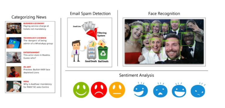
Benefit: Bayesian methods, such as Naive Bayes, handle sparse data well and provide probabilistic interpretations of classifications.
The general form of the Naive Bayes conditional independence assumption can be expressed mathematically as:
\[
P(C | X_1, X_2, \ldots, X_n) = \frac{P(C) \cdot \prod_{i=1}^{n} P(X_i | C)}{P(X_1, X_2, \ldots, X_n)}
\]
Here:
The product operator \(\prod_{i=1}^n\) indicates that you multiply the likelihoods of the individual features given the class CCC. This is a key part of the Naive Bayes assumption, which assumes that the features are conditionally independent given the class.
In simpler terms, the symbol “\(\prod\)” in this context tells you to take the product of the probabilities of each feature \(X_i\) occurring given the class \(C\), and this product is then combined with the prior probability of the class CCC to compute the posterior probability.
4. Robotics
Use Case: Path planning and localization.
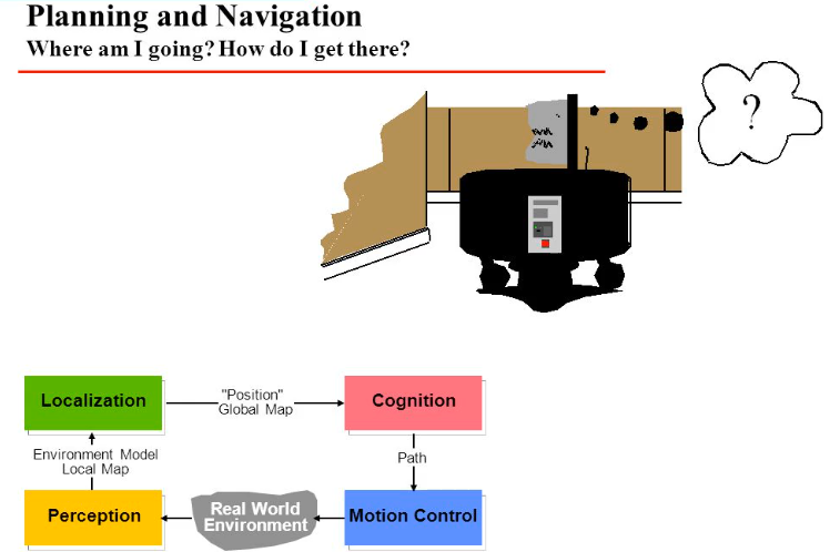
Benefit: Bayesian methods can model the uncertainty in sensor data and the environment, leading to more robust decision-making.
For example, estimating the robot’s position given sensor readings \(P(X \mid S)\):
\[ P(X | S) = \frac{P(S | X) P(X)}{P(S)} \]
5. Marketing and Customer Segmentation
Use Case: Predicting customer behavior and segmenting markets.
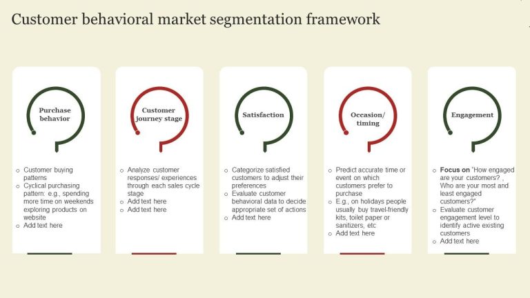
Benefit: Bayesian methods can incorporate prior market knowledge and continuously update segmentation models as new data is collected.
For example, segmenting customers based on purchase history \(P(C \mid H)\):
\[ P(C | H) = \frac{P(H | C) P(C)}{P(H)} \]
Bayesian Machine Learning offers a robust framework for incorporating uncertainty and prior knowledge into machine learning models. By leveraging probabilistic methods, Bayesian approaches provide a more nuanced understanding of model parameters and their distributions, leading to better decision-making and more interpretable results.
Bayesian methods, while computationally intensive, offer significant advantages, especially in scenarios where uncertainty is paramount. As computational resources and algorithms improve, the application of Bayesian techniques is likely to become more prevalent in the machine learning community. The ability to continuously update models with new data and incorporate prior knowledge makes Bayesian Machine Learning a valuable tool for a wide range of applications.
As Tech Co-Founder at Yugensys, I’m passionate about fostering innovation and propelling technological progress. By harnessing the power of cutting-edge solutions, I lead our team in delivering transformative IT services and Outsourced Product Development. My expertise lies in leveraging technology to empower businesses and ensure their success within the dynamic digital landscape.
Looking to augment your software engineering team with a team dedicated to impactful solutions and continuous advancement, feel free to connect with me. Yugensys can be your trusted partner in navigating the ever-evolving technological landscape.

Linkedin Instagram Facebook X-twitter Case Study Automating the generation of javascript expressions with Pre-Trained AI Models Challenge Developing a user-friendly…

Linkedin Instagram Facebook X-twitter In today’s tech landscape, harnessing the capabilities of artificial intelligence (AI) is pivotal for creating innovative…

Linkedin Instagram Facebook X-twitter Welcome to our comprehensive guide on bundling a React library into a reusable component library! In…
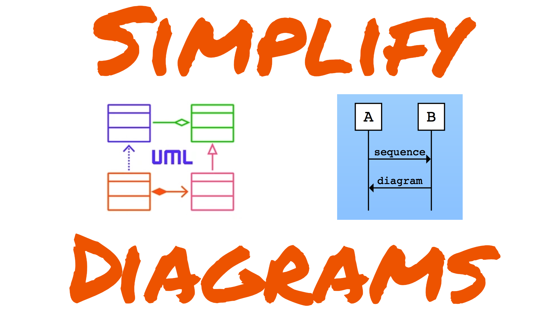
Linkedin Instagram Facebook X-twitter In today’s tutorial, we’ll explore creation of stunning diagrams using ChatGPT, along with the assistance of…