Ant Colony Optimization Explained: A Nature-Inspired Solution for Complex Problems
Table of Contents
Navigating through a grid filled with obstacles might sound challenging, but with propositional logic, AI agents can make intelligent, rule-based decisions at every step. Imagine guiding a robot across a grid, avoiding obstacles, and achieving a specific goal – all powered by logical reasoning.
Why It’s Important: Propositional logic is foundational for many AI systems, particularly in scenarios requiring structured decision-making, like grid navigation. By understanding these basics, beginners can explore more advanced AI applications, from robotics to natural language processing.
What You’ll Learn: This guide will introduce you to propositional logic and its application in AI for grid-based navigation, centered on a knowledge-based agent. The entire expert-written content, including mathematical expressions and examples, is preserved here for an in-depth understanding.
Introduction
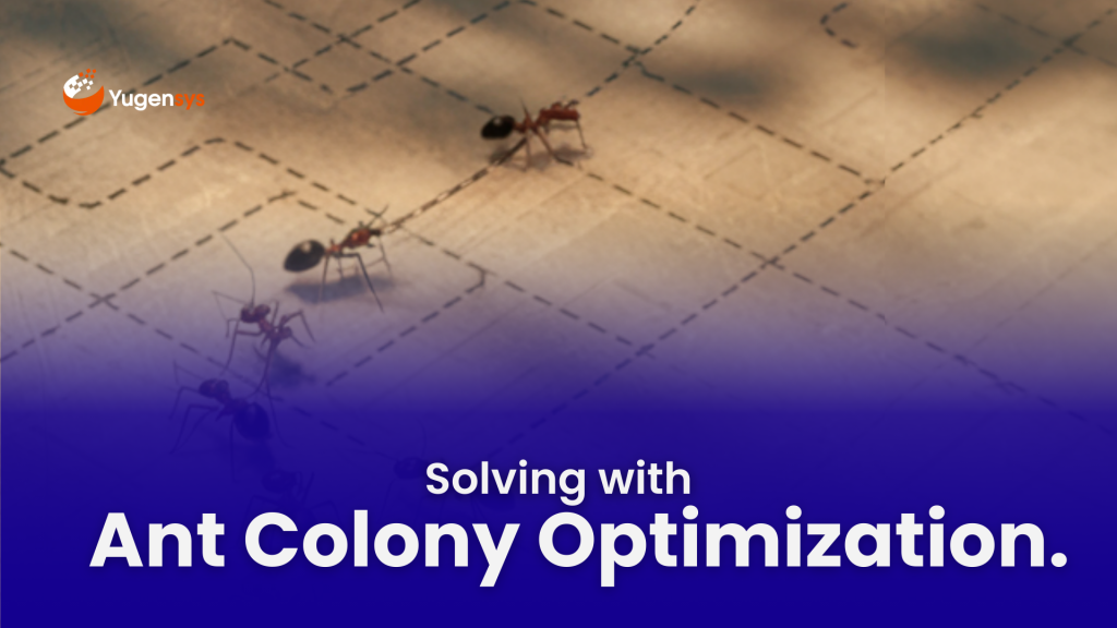
Ant Colony Optimization (ACO) is a popular nature-inspired algorithm designed to solve complex optimization problems. Modeled after the foraging behavior of ants, ACO has found widespread applications in solving problems such as the Traveling Salesperson Problem (TSP), vehicle routing, and network optimization. In this blog post, we’ll explore how ACO works, the detailed steps involved, and a practical application with code to solve a real-world problem.
Why Ant Colony Optimization Matters
Optimization problems are at the heart of many real-world applications, such as:
- Logistics and transportation: Efficiently routing vehicles or goods.
- Telecommunications and networks: Designing robust, scalable networks.
- Manufacturing: Improving production schedules and supply chain efficiency.
Traditional approaches often struggle with these large-scale, complex problems due to their computational costs. ACO provides a heuristic, metaheuristic approach that is not only scalable but also computationally efficient. Its relevance grows in scenarios where real-time decisions are critical.
How Ant Colony Optimization Works
ACO mimics the pheromone-laying and following behavior observed in ant colonies:
- Initialization: Artificial ants start at random positions and traverse the search space.
- Heuristic building: Paths are constructed based on pheromone levels and heuristic desirability (like inverse distance in TSP).
- Pheromone updating: Successful paths receive more pheromones, reinforcing the probability of future ants following them.
- Evaporation: Pheromones decay over time to prevent premature convergence to suboptimal solutions.
For example, in solving the TSP, ACO ants iteratively construct tours between cities, reinforcing shorter paths with more pheromones while exploring new possibilities.
Problem Statement
Optimization problems are pervasive in various domains, including logistics, network design, and operations research. One of the most well-known examples is the Traveling Salesperson Problem (TSP), where the goal is to find the shortest possible route that visits a set of cities exactly once and returns to the starting point. Given the problem’s NP-hard nature, exact methods become impractical for large instances, necessitating the use of heuristic or metaheuristic approaches like ACO.
In this blog, we will focus on how Ant Colony Optimization can be applied to solve the TSP by mimicking the pheromone-laying and following behaviour of ants in nature.
How Ant Colony Optimization Solves the Problem
Ant Colony Optimization is based on the collective intelligence of ants. When searching for food, ants deposit pheromones along their path, which serve as a signal to other ants. Over time, paths with higher pheromone concentrations attract more ants, reinforcing the route to the food source. This collective learning process helps the colony find the shortest path to the food.
In the context of optimization, artificial ants traverse the solution space and build solutions incrementally based on pheromone levels and a problem-specific heuristic.
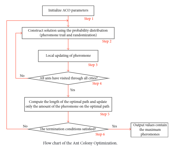
Problem Setup
We have a small TSP with 4 cities. The distances between cities are given by the following distance matrix:
\[x = \begin{bmatrix} 0 & 2 & 9 & 10 \\ 1 & 0 & 6 & 4 \\ 15 & 7 & 0 & 8 \\ 6 & 3 & 12 & 0 \end{bmatrix}\]
Step 1: Initialization
- Number of ants (m) = 4 (equal to the number of cities)
- Number of cities (n) = 4
- Initial pheromone levels \( \tau_{ij} \) are uniformly set, say \( \tau_{ij} \) = \(1 \quad \text{for all } i, j\)
- Parameters: \(α=1\) (importance of pheromone), β=2 (importance of distance), \(ρ=0.5\)
(evaporation rate).
Step 2: Ant Movement and Probability Calculation
Each ant starts from a different random city and constructs a tour by moving to unvisited cities based on the probability Pij of moving from city i to city j.
The probability Pij is calculated using the formula:
\[P_{ij} = \frac{[\tau_{ij}]^\alpha \times [\eta_{ij}]^\beta}{\sum_{k \in \text{allowed}} [\tau_{ik}]^\alpha \times [\eta_{ik}]^\beta}\]
where \(\eta_{ij} = \frac{1}{d_{ij}}\) is the visibility or the inverse of the distance between city i and city j.
For example, if an ant starts at city 1, the probability of moving to city 2 is calculated as follows:
- Pheromone level: \(τ_{12} = 1\)
- Distance: \(d_{12} = 2\)
- Visibility: \(\eta_{12} = \frac{1}{2} = 0.5\)
The probability \(P_{12}\) is:
\[P_{12} = \frac{\sum_{k \in \{2,3,4\}} \tau_{1k}^{\alpha} \times \eta_{1k}^{\beta}}{\tau_{12}^{\alpha} \times \eta_{12}^{\beta}}\]
\[P_{12} = \frac{1 \times \left(\frac{1}{d_{12}}\right)^{\beta}}{0.25 + \left(\frac{1}{9}\right)^{2} + \left(\frac{1}{10}\right)^{2}}\]
\[P_{12} = \frac{0.25}{0.25 + 0.0123 + 0.01} \approx \frac{0.25}{0.2723} \approx 0.918\]
Similarly, the probabilities \(P_{13}\) and \(P_{14}\) are calculated.
Step 3: Update Pheromones
After all ants have completed their tours, the pheromone levels are updated. The pheromone on each edge is updated using the formula:
\[\tau_{ij}(t+1) = (1 – \rho) \times \tau_{ij}(t) + \Delta \tau_{ij}\]
where \(\Delta \tau_{ij}^{\text{ant}}\) is the pheromone deposited by each ant, inversely proportional to the tour length \(L_{\text{ant}}\) of the ant that traveled that path:
\[\Delta \tau_{ij}^{\text{ant}} = \frac{Q}{L_{\text{ant}}}\]
If an ant completes a tour of length 25, the pheromone deposition might be:
\[\Delta \tau_{ij}^{\text{ant}} = \frac{1}{25} = 0.04\]
Step 1: Initialization
Step 2: Ant Movement and Probability Calculation
Each ant starts from a different random city and constructs a tour by moving to unvisited cities based on the probability Pij of moving from city i to city j.
The probability Pij is calculated using the formula:
\[P_{ij} = \frac{[\tau_{ij}]^\alpha \times [\eta_{ij}]^\beta}{\sum_{k \in \text{allowed}} [\tau_{ik}]^\alpha \times [\eta_{ik}]^\beta}\]
where \(\eta_{ij} = \frac{1}{d_{ij}}\) is the visibility or the inverse of the distance between city i and city j.
For example, if an ant starts at city 1, the probability of moving to city 2 is calculated as follows:
- Pheromone level: \(τ_{12} = 1\)
- Distance: \(d_{12} = 2\)
- Visibility: \(\eta_{12} = \frac{1}{2} = 0.5\)
The probability \(P_{12}\) is:
\[P_{12} = \frac{\sum_{k \in \{2,3,4\}} \tau_{1k}^{\alpha} \times \eta_{1k}^{\beta}}{\tau_{12}^{\alpha} \times \eta_{12}^{\beta}}\]
\[P_{12} = \frac{1 \times \left(\frac{1}{d_{12}}\right)^{\beta}}{0.25 + \left(\frac{1}{9}\right)^{2} + \left(\frac{1}{10}\right)^{2}}\]
\[P_{12} = \frac{0.25}{0.25 + 0.0123 + 0.01} \approx \frac{0.25}{0.2723} \approx 0.918\]
Similarly, the probabilities \(P_{13}\) and \(P_{14}\) are calculated.
Step 3: Update Pheromones
After all ants have completed their tours, the pheromone levels are updated. The pheromone on each edge is updated using the formula:
\[\tau_{ij}(t+1) = (1 – \rho) \times \tau_{ij}(t) + \Delta \tau_{ij}\]
where \(\Delta \tau_{ij}^{\text{ant}}\) is the pheromone deposited by each ant, inversely proportional to the tour length \(L_{\text{ant}}\) of the ant that traveled that path:
\[\Delta \tau_{ij}^{\text{ant}} = \frac{Q}{L_{\text{ant}}}\]
If an ant completes a tour of length 25, the pheromone deposition might be:
\[\Delta \tau_{ij}^{\text{ant}} = \frac{1}{25} = 0.04\]
Application of Steps: Solving the TSP
Let’s apply ACO to solve the TSP using the example above. In the first iteration:
- Initialization:
- Each ant starts at a different city.
- Initial pheromone levels are set uniformly to, \(u_{ij}\) = 1
- \(α=1, β=2, ρ=0.5\).
- Movement:
- Each ant probabilistically chooses the next city based on the pheromone and visibility.
- After visiting all cities, the ant completes a tour.
- Pheromone Update:
- Pheromone levels are updated based on the length of each ant’s tour.
- Paths that are part of shorter tours receive more pheromone, increasing the likelihood of being chosen in future iterations.
- Repeat:
- Repeat the construction and updating steps for a set number of iterations or until convergence.
Sample Implementation
Here’s an example Python code snippet implementing ACO for TSP:
Detailed Statistics:
import numpy as np
# Define distance matrix
dist_matrix = np.array([
[0, 2, 9, 10],
[1, 0, 6, 4],
[15, 7, 0, 8],
[6, 3, 12, 0]
])
# Initialize parameters
num_ants = 4
num_cities = dist_matrix.shape[0]
alpha = 1.0
beta = 2.0
rho = 0.5
num_iterations = 100
pheromone = np.ones_like(dist_matrix)
def ant_colony_optimization():
for _ in range(num_iterations):
paths = []
for ant in range(num_ants):
path = [np.random.randint(num_cities)]
for _ in range(num_cities – 1):
next_city = select_next_city(path, pheromone, dist_matrix, alpha, beta)
path.append(next_city)
paths.append(path)
update_pheromones(paths, pheromone, dist_matrix, rho)
return pheromone
#Implement select_next_city and update_pheromones functions as per ACO steps
optimized_pheromones = ant_colony_optimization()
| Parameter | Value |
|---|---|
| Initial Pheromone Level, τij0 | 1 |
| Distance between nodes dij | 1.05, 9.10 |
| Heuristic information ηij | 1.2, 0.11, 0.10 |
| Transition Probability Pij | 0.958 |
| Pheromone Update Δτij | 0.04 |
This table represents the critical values calculated during the first iteration of the Ant Colony Optimization algorithm, including the pheromone levels, distances, heuristic values, and probabilities.
Impact of Varying Parameters
Effect of α and β:
- α: Controls the influence of the pheromone trail on the decision-making process. A higher α value makes the algorithm more reliant on pheromone concentration, potentially leading to faster convergence but higher risk of getting trapped in local optima.
- β: Determines the importance of heuristic information (e.g., distance). A higher β value emphasizes the heuristic, encouraging exploration of shorter paths initially.
By experimenting with different α and β values, you can balance the exploration and exploitation trade-off. For instance, a higher β could be beneficial in the early stages of the algorithm to explore diverse solutions, while increasing α later can help in intensifying the search around promising areas.
Influence of Evaporation Rate ρ:
- ρ: The pheromone evaporation rate prevents the algorithm from prematurely converging by reducing the influence of older pheromone trails. A higher ρ accelerates evaporation, encouraging exploration, but if too high, it can lead to loss of useful pheromone information, making it harder for the ants to find an optimal path.
Initial Pheromone Level \(τ_0\):
The initial pheromone level can significantly influence the early convergence behavior. If τ0 is set too high, the ants may quickly converge on suboptimal paths. Setting it too low, however, might slow down the convergence process, as the pheromone trails may not have enough influence on ant decisions.
Iterative Improvement Over Multiple Iterations
The algorithm refines its solution over multiple iterations. Each iteration allows ants to update the pheromone trails based on the quality of their paths. Over time, this iterative process helps in gradually improving the solution, as paths that are part of shorter tours accumulate more pheromone, increasing their likelihood of being chosen in subsequent iterations
Additional Analysis
- Convergence Analysis: Track how the best solution evolves over iterations to analyze the algorithm’s convergence behavior.
- Diversity Maintenance: Monitor how diverse the solutions are in different iterations to ensure the algorithm explores the solution space adequately before converging.
Conclusion
Ant Colony Optimization is an effective algorithm for solving the Traveling Salesman Problem by leveraging the collective intelligence of ants. Through the interaction of pheromone trails and probabilistic decision-making, ACO converges towards an optimal or near-optimal solution over multiple iterations. The method balances exploration of new paths and exploitation of known good paths, making it robust for various optimization problems.
As the Tech Co-Founder at Yugensys, I’m driven by a deep belief that technology is most powerful when it creates real, measurable impact.
At Yugensys, I lead our efforts in engineering intelligence into every layer of software development — from concept to code, and from data to decision.
With a focus on AI-driven innovation, product engineering, and digital transformation, my work revolves around helping global enterprises and startups accelerate growth through technology that truly performs.
Over the years, I’ve had the privilege of building and scaling teams that don’t just develop products — they craft solutions with purpose, precision, and performance.Our mission is simple yet bold: to turn ideas into intelligent systems that shape the future.
If you’re looking to extend your engineering capabilities or explore how AI and modern software architecture can amplify your business outcomes, let’s connect.At Yugensys, we build technology that doesn’t just adapt to change — it drives it.
Subscrible For Weekly Industry Updates and Yugensys Expert written Blogs
